Authors: Ethan Senatore, Vineet Pasumarti, Allen Zhou, Raymond Yang
In our first lab session, we implemented both a controller and waypoint planner on a CrazyFlie 2.0. We first validated the quadrotor's stability with a hover, then tuned our controller's $z$ position gain using an altitude step response. We then tuned $x$ and $y$ position gains using a lateral step response. We evaluated our controller against a test "box" maneuver, and with our extra lab time we wrote our own test waypoints to fly the drone in a rectangular spiral and land.
In our second lab session, we deployed our stack on the CrazyFlie to plan a path through a maze and execute the resulting trajectory. This required us to re-evaluate our gains and fine-tune the margins of our occupancy map to ensure the safe traversal of the drone from start to finish. Following both sessions, we were able to demonstrate successful control and flight path generation. Tuning parameters on real hardware allowed us to be less risk-averse and execute more aggressive trajectories that navigate the cluttered environment faster and smoother.
The CrazyFlie 2.0 is a palm-sized quadrotor that we cover with markers to be tracked by a VICON system. VICON is a motion capture system that uses multiple infrared cameras to track the position and orientation of an object. The quadrotor's position and orientation are tracked by the VICON and the angular velocity and acceleration from the onboard accelerometer and gyroscope are all radio transmitted to the lab computers. This information is fed to our controller as an input, which runs on the lab computers to generate a desired state and the necessary motor commands are then transmitted back to the quadrotor.
The controller we elected to use for our experiments was a geometric nonlinear controller. In an intuitive sense, the controller is structured around the idea of orienting the quadrotor's z-axis in the direction we desire to move to. This controller allows for aggressive maneuvers and requires fine-tuning of both the damping and gain. Using the Project 1.1 handout as a reference, we will define the theoretical framework of the controller. We start with the PD controller equation:
$$\ddot{r}^{des} = \ddot{r}_T - K_d(\dot{r}-\dot{r}_T) -K_p(r-r_T)$$
To compute the inputs $u_1$ and $u_2$ in order to generate our desired acceleration we use the following equation:
$$m\ddot{r}^{des} + \begin{bmatrix} 0\\0\\mg \end{bmatrix} = u_1R\begin{bmatrix} 0\\0\\1 \end{bmatrix}$$
We can identify that the left hand side of the equation is simply the desired force combined with the gravitational force. Thus, we can simplify the equation in order to solve for $u_1$ as follows:
$$F^{des} = m\ddot{r}^{des} + \begin{bmatrix} 0\\0\\mg \end{bmatrix}$$ $$u_1 = \begin{bmatrix} 0\\0\\1 \end{bmatrix}^T R^T F^{des}$$
Calculating $u_2$ requires a slightly more complex process. Based off of the previously laid out intuition, we seek to align the thrust vector with the quadrotor's z-axis. Thus,
$$c_3^{des} = \frac{F^{des}}{||F^{des}||}$$
Next, we seek to align the quadrotor's y-axis with the desired yaw direction while maintaining the orthogonality between the y and x-axes. To do so, we first define the following term:
$$a_\psi = \begin{bmatrix} \cos\psi_T\\\sin\psi_T\\0 \end{bmatrix}$$
this vector represents the yaw direction in the world x-y plane. Next, we can calculate the y-axis vector as follows:
$$c_2^{des} = \frac{c_3^{des}\times a_\psi}{||c_3^{des}\times a_\psi||}$$
Finally, we can define the desired $R^{des}$
$$R^{des} = \begin{bmatrix} c_2^{des} \times c_3^{des}, & c_2^{des}, & c_3^{des} \end{bmatrix}$$
This rotation matrix represents the desired orientation we wish to achieve at a given time step. The next step is to measure the error between our current and desired orientation.
$$e_R = \frac{1}{2}(R^{des^T}R - R^TR^{des})^\vee$$
Another aspect of control we may care about is the difference between our desired and current angular velocities. We can easily define this term as:
$$e_\omega = \omega - \omega^{des}$$
Finally, we can define $u_2$ as:
$$u_2 = I(-K_Re_R - K_\omega e_\omega)$$
Using this controller, we have four tunable gains that we had to first meticulously tune in simulation and then finalize in our experiments. After tuning our controller, in simulation, lab 1, and lab 2 we settled on the following configuration. The 1x3 vector listed in Table I represents the diagonal of a 3x3 matrix.
| Gain | Value | Units |
|---|---|---|
| $K_p$ | [2.45, 2.45, 10.5] | 1/$s^2$ |
| $K_d$ | [5.25, 5.25, 6.3] | 1/$s$ |
| $K_R$ | [1750, 1750, 140] | 1/$s^2$ |
| $K_\omega$ | [175, 175, 105] | 1/$s$ |
Intuitively, we interpreted the gains as ways to answer four different questions. Starting with $K_p$, we viewed this metric as measuring 'how important is it to to achieve a desired position?'. $K_d$ is the measure of 'how fast do you want to get to the desired position?'. Similarly, we can say that $K_R$ measures 'how important is it to achieve a desired orientation?' and $K_\omega$ measures 'how fast do you want to achieve the desired orientation?'. This intuition provided us a steady foundation to work off of and fine tune our parameters. It was fairly easy to tinker with each gain to reach our desired performance. However, we immediately noticed that testing on hardware required us to scale down our gains by around 30%. Additional fine-tuning during lab 1 and 2 narrowed us down to our final parameters. We can attribute the differences in gains due to model mismatch, lack of simulation fidelity, and flaws in our controller implementation.

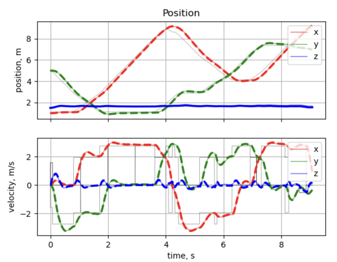
Figure I shows an experiment we ran to tune our y-direction gain and damping parameters. Based on the plots, we can determine that our controller demonstrates a settling time of around 2 s, a rise time of around 1.1 s, a steady state error of around 2%, and a damping ratio of around 0.4. This experiment revealed a few flaws in our controller. First and foremost, the controller is underdamped and takes fairly long to settle into a steady state. Secondly, we immediately recognized a glaring issue in our z-direction tuning. At first, we attributed the discrepancy in desired and actual position as model mismatch, but in lab 2 we retuned our z gains to fix this issue. The process of fine-tuning the gains was straightforward as we would conduct a test, adjust the parameters, and repeat until we were satisfied.
In this section, we discuss the approach for the generation of a piecewise trajectory connecting the waypoints from start to target for an input map in the discretized occupancy grid, as well as a method that generates an optimized flight path that aligns with the quadrotor's maneuverability while maintaining collision-free.
Starting with the default occupancy_map file where a 3D occupancy map is generated
from the given map environment by splitting the space into a grid of voxels at a given axial
resolution, the occupancy map consists of voxels that are marked "occupied" when they intersect
an obstacle or hit the boundary within the workspace, and others representing the discretized
waypoints that are open access to the graph search planner.
Then, the graph_search treats each unoccupied voxel from the previous map as a node
in a graph, which is able to develop up to 26 edges connecting its neighbors in 3D. During the
lab execution, an A* graph search algorithm is preferred over the plain Dijkstra method, since
it incorporates a heuristic measure, which is the straight-line distance to the goal, to guide
the search more efficiently. This heuristic attracts the exploration toward the target node,
significantly reducing the exploration time to find an optimal path compared to Dijkstra, which
blindly develops its path outward. To conclude, the cost of moving between neighboring nodes is
the Euclidean distance [$l_2$ norm], while an admissible heuristic $h(n)$ estimates the cost
from the current node to the goal.
$$c(\text{current}, \text{neighbor}) = \|\text{neighbor} - \text{current}\|$$ $$h(n) = \|n - \text{goal}\|$$
The total cost at each node is therefore:
$$f(n) = g(n) + h(n)$$
where $g(n)$ represents the cost so far from the start node to the current.
After running A*, we apply the Ramer-Douglas-Peucker (RDP) algorithm to reduce redundant points along nearly straight segments. An RDP tolerance of $\varepsilon = 0.1\text{ m}$ is used, which prunes interior waypoints whose perpendicular distance to the line between the first and last point in a subset is below $\varepsilon$. The outcome is a sparser set of critical waypoints, preserving the overall path shape but removing unnecessary intermediate points that might complicate maneuvering along the trajectory. We construct a piecewise linear position trajectory to connect along each optimized waypoint, commanding the quadrotor to operate from start to goal. The position where each single segment ends is:
$$\mathbf{x}(t) = \mathbf{p}_i + (\mathbf{v}_i)(t - t_{\mathrm{start},i}), \quad t \in [t_{\mathrm{start},i}, t_{\mathrm{start},i} + T_i]$$
where $\mathbf{v}_i$ is a constant velocity vector for segment $i$, defined by
$$\mathbf{v}_i = v_i \frac{\mathbf{p}_{i+1} - \mathbf{p}_i}{\|\mathbf{p}_{i+1} - \mathbf{p}_i\|}$$
Hence, velocity is constant in each segment, and the position changes linearly from $\mathbf{p}_i$ to $\mathbf{p}_{i+1}$. Once $t$ exceeds $t_{\mathrm{start},i}+T_i$, we switch to the next segment $i+1$ until the Crazyflie hits the target. In our code, $v_i$ is chosen based on the segment length and the angular change between consecutive segments (with mild speed reductions if there is a sharp turn). The total trajectory time becomes
$$T_{\mathrm{total}} = \sum_{i=0}^{N-1} T_i$$
where a constant speed $v_i$ for each segment $[\mathbf{p}_i \rightarrow \mathbf{p}_{i+1}]$ is:
$$T_i = \frac{\|\mathbf{p}_{i+1} - \mathbf{p}_i\|}{v_i}$$
Since each segment uses constant velocity, the overall trajectory is only continuous in position
($C^0$-continuous); velocity changes instantaneously at segment boundaries. However, we limit
the speed of the Crazyflie to under 1 m/s, which prevents aggressive maneuvering during the
tests. By including an obstacle inflation margin of $0.2\text{ m}$ and a resolution of the
occupancy grid of $\Delta x = \Delta y = \Delta z = 0.25\text{ m}$, we ensure that the resulting
waypoints remain safely away from obstacles while keeping a low computational load. Hence, while
the piecewise-linear approach does not strictly enforce higher-order continuity, it is
straightforward to implement, fast to compute, and guarantees collision-free given the flight
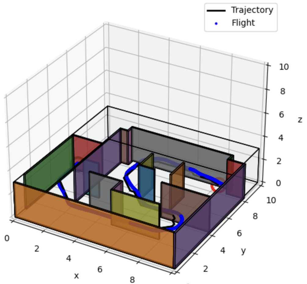
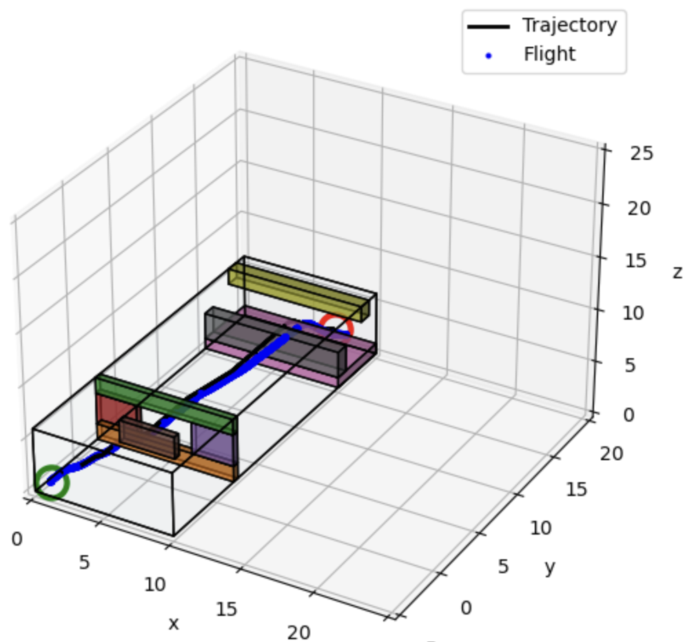
map. The plots below show (1) discrete waypoints and path, (2) 3D quadrotor trajectory, and (3)
position, velocity, and acceleration log in the map maze_2025_1.


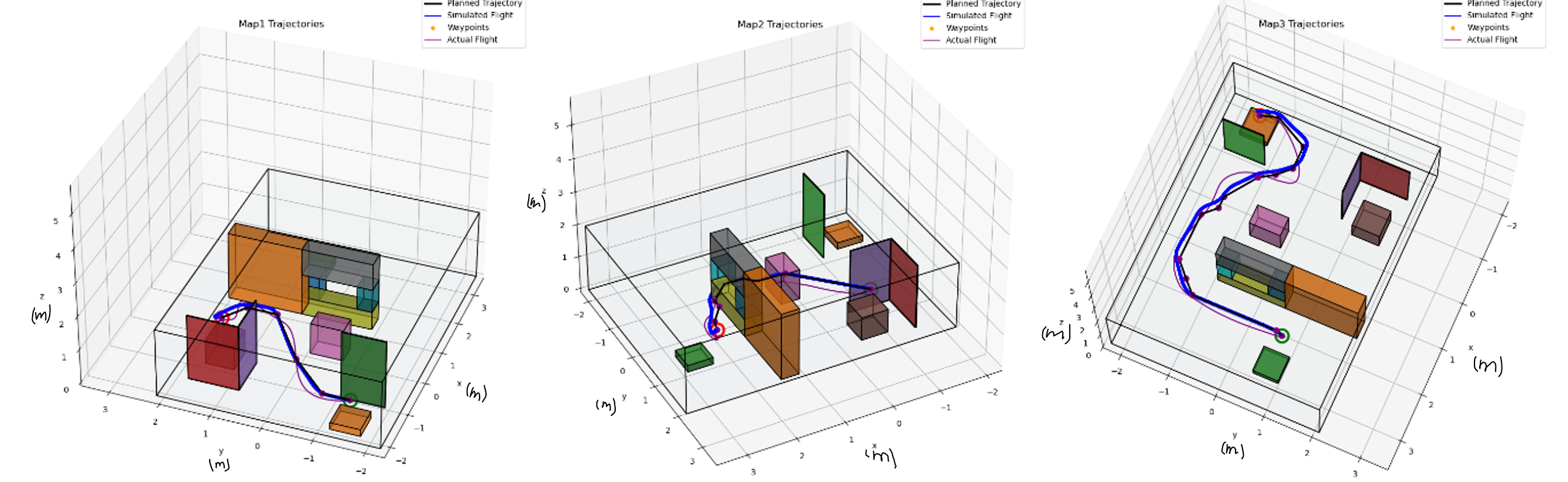

We observe discrepancies between the planned trajectory and actual flight path in all three maps, especially during sharp turns and maneuvers around obstacles. One possible cause for the tracking error comes from the motor thrust limitations. The maximum thrust capabilities of the flight motors restricted the drone's response to control inputs during high-demand maneuvers, leading to larger than anticipated deviations from the planned path. In addition, interruptions in positional data due to occlusions of VICON cameras by obstacles resulted in inaccurate state estimations, causing the drone to stray off course. The discrepancies between the simulated and actual weight of the drone can be another cause, it led to inadequate PID controller settings and impacting the drone's dynamic response to control commands. To achieve safe trajectories, we can directly adjust the trajectory planning algorithm to include larger safety margins around obstacles, accounting for potential hardware limitation during path planning. We can also further adjust PID parameters using actual drone weight data.
Since we have already observed undesired flight paths, it can be dangerous to make the trajectory more aggressive. The limited maximum thrust of the flight motors restricted the drone's ability to execute rapid or steep maneuvers, essential for more aggressive trajectories. The observed inaccuracies in positional data due to VICON camera occlusions and the lack of precise PID tuning for the actual drone weight meant that increasing the aggressiveness of the trajectories could lead to higher risks of collision or loss of control.
To improve the system reliability and speed, one change we can make is tune the PID using real world data to reduce the discrepancy between simulated trajectory and actual pathways. A more robust trajectory planning algorithm can also improve the system reliability and speed, with higher dimension spline fitting, the trajectory can be smooth and reduce the potential issue with motor torque limitations. Incorporate higher resolution in path planning is another effective approach to enhance both the speed and reliability of the drone system. This allows the trajectory to be optimized at a more detailed level, enabling smoother transitions and tighter navigation around obstacles.
If we had one more session in the lab to do something interesting, it will be interesting to try implementing more advanced control techniques with PID controller parameters dynamically based on observed performance metrics and environmental conditions encountered during flight. The goal would be to see how well the drone can optimize its flight stability and accuracy in response to dynamically changing conditions within the maze, potentially leading to more reliable and efficient navigation.
In this project, we develop a full autonomy stack that plans a path using the A* graph search algorithm, sparsifies waypoints according to the Ramer–Douglas–Peucker algorithm and generates a smooth trajectory for minimum jerk, completes the trajectory using a quadrotor PD controller, and relies solely on visual inertial odometry (VIO) using Error State Extended Kalman Filtering (ES-EKF) for on-board state estimation.
The problem at hand differs from Project 1 due to our previous dependency on the VICON motion capture system to track position and orientation when we deployed to real hardware. Although position and orientation can be obtained through strapdown integration of the angular velocity and linear acceleration data from the IMU, this computation accumulates sensor biases and is prone to drift. Additionally, double-integration of accelerometer data implies the position error increases quadratically with time.
We resolve this problem by implementing stereo vision in conjunction with an IMU to estimate the state using an ES-EKF. Stereo vision allows us to track features and predict the quadrotor's transformations according to feature correspondences, as well as estimate the absolute depth of a feature by measuring the disparity across rectified images from both cameras. By optimally combining our various state estimates in an ES-EKF, the addition of stereo vision will reduce the covariance of the state vector and lead to a better estimate of position and orientation, allowing for the quadrotor to navigate an environment using only on-board sensors.
Previously, we relied on a ground truth mechanism to provide the state of the quadrotor. In practice, this meant tracking the position and orientation with a VICON motion capture system and processing the angular velocity and acceleration from the on-board accelerometer and gyroscope. In this project, we utilize stereo vision in conjunction with the IMU to estimate the state of the quadrotor. We achieve this by combining multiple estimates optimally using an ES-EKF.
Both Extended Kalman Filters (EKF) and Unscented Kalman Filters (UKF) are standard choices for systems that adhere to nonlinear dynamics and/or nonlinear observations. The EKF is an optimal estimator for nonlinear systems up to the first order, and is preferable due to its simplicity and similarity to the standard Kalman Filter. However, the EKF requires that all components of the state be isomorphic in Euclidean vector space, such that the state vector can iteratively be summed linearly at each time step to obtain an optimal estimate. Therefore, a standard EKF cannot include orientation in the state vector as directly adding quaternions results in arbitrary 4x1 vectors. For this reason, we opt to use an ES-EKF that instead iterates upon the error state of the state vector, which can be represented in the Euclidean vector space. At each time step, we update the nominal state by propagating the dynamics of the quadrotor according to the linear acceleration and angular velocity as obtained by the IMU. We then propagate the error state covariance matrix which represents the uncertainty in our current estimation error for the position, velocity, orientation, accelerometer and gyroscope biases, and gravity vector. We optimally propagate the error state covariance matrix according to the following equation,
$$P=F_x P F_x^{\top}+F_i Q_i F_i^{\top}$$
where $F_x$ and $F_i$ are the state transition Jacobians with respect to the error and perturbation vectors, and $Q_i$ is the process noise covariance matrix. Lastly, we update our nominal state estimate and error state using an image measurement, $uv$, which is a 2D projection of a known world point in 3D. The difference between $uv$ and the transformed world point is the innovation, $I$. We then compute the Kalman Gain, $K$,
$$K=P H^{\top}\left(H P H^{\top}+Q\right)^{-1}$$
where $Q$ denotes the covariance matrix of the image measurement $uv$ and $H$ represents the measurement Jacobian. We compute the error state, $KI$, as well as update the error state covariance matrix, $P$.
$$P \leftarrow(I-K H) P(I-K H)^{\top}+K Q K^{\top}$$
This implementation of the EKF allows us to update the state of the quadrotor optimally using both visual and inertial information.
When directly implementing the VIO-based estimate alongside the original project 1 code, we find that the drone often hovers adjacent to the goal location indefinitely, despite being away from the planned trajectory. We observe this in Figures VII and VIII, as the quadrotor appears to be at the goal location, yet the simulation ultimately times out as the sensor readings continue until 150 seconds.
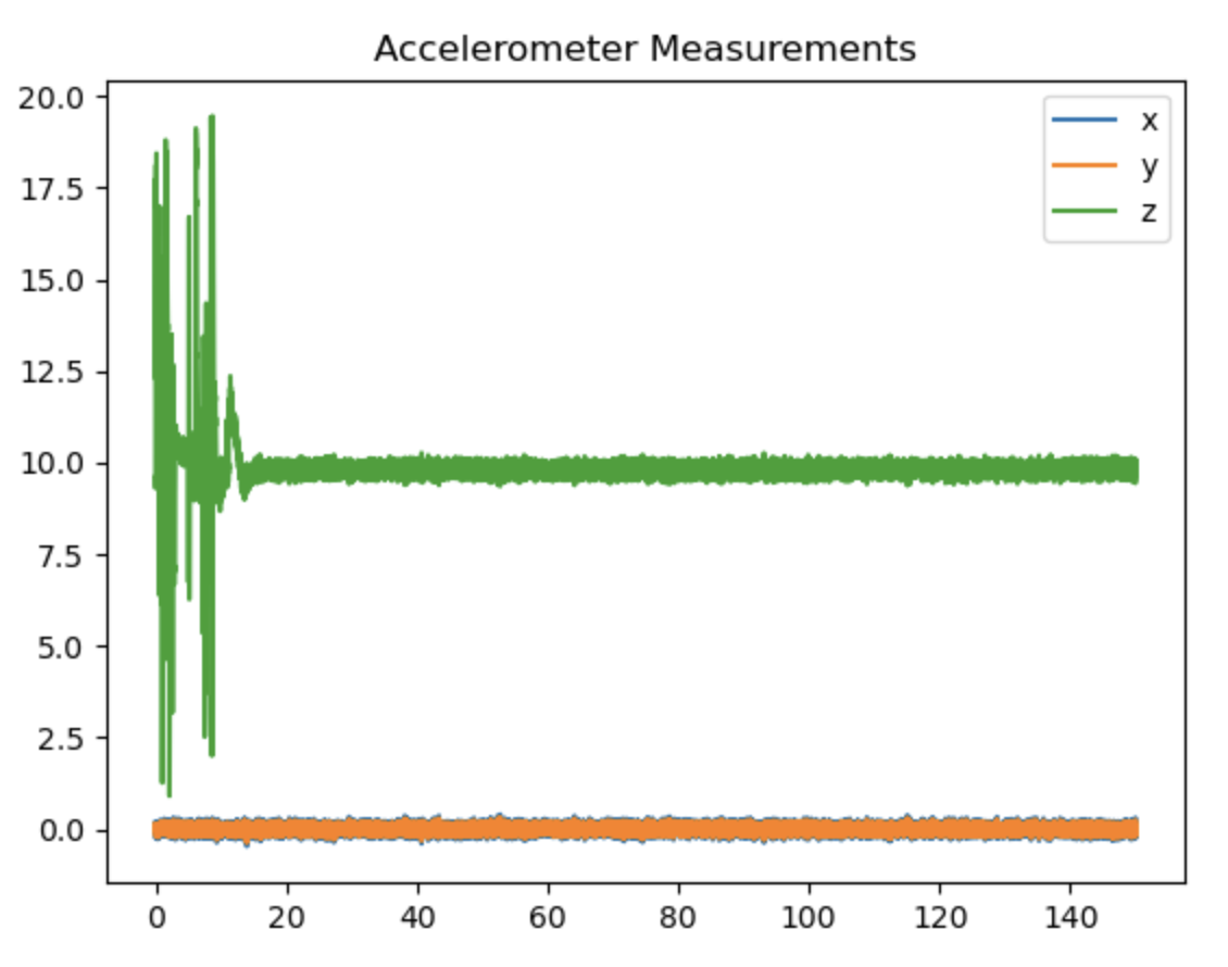
Confidently estimating an incorrect state is dangerous. We can take advantage of Kalman Filtering by artificially increasing the accelerometer and gyroscope covariance to influence the Kalman gain. Increasing the noise and random walk terms in the IMU's process noise covariance matrix, $Q_i$, effectively informs the EKF that the inertial predictions are less reliable and gives more weight to the stereo vision measurements to correct its state. We find that scaling up the IMU noise and random walk terms in the process noise covariance matrix by 9 works well in the example test cases. During the EKF update, a larger $Q_i$ due to the intentional scaling yields a larger $P$, so $K$ increases and the EKF places more weight on stereo vision measurements over the IMU prediction. This strategy shows success in the automated test cases as the quadrotor completes the desired trajectory within reasonable time and no longer hovers adjacent to the goal location indefinitely.
We make an additional change to the existing code base in this project. Although we continue to implement a geometric nonlinear PD controller for the quadrotor, we modify the gains to more accurately follow the minimum jerk trajectory. We opt to use the following gains as shown in Table II, where the 1x3 vector of values are representative of the diagonal of a 3x3 matrix.
| Gain | Value | Units |
|---|---|---|
| $K_p$ | [4.2, 4.2, 8.4] | 1/$s^2$ |
| $K_d$ | [9, 9, 7.2] | 1/$s$ |
| $K_R$ | [3000, 3000, 240] | 1/$s^2$ |
| $K_\omega$ | [300, 300, 180] | 1/$s$ |
The gains in Table II are roughly 1.2x the gains used in project 1.3. We find that the drone's tendency to undershoot the desired position is exacerbated when using an ES-EKF to fuse the IMU and stereo vision state estimates. As a result, the quadrotor initially had a tendency of colliding despite being provided an obstacle-free trajectory with generous margins (0.5m). By uniformly increasing the proportional and derivative gains, the quadrotor tracks the trajectory more aggressively without encountering oscillations. Scaling up proportional gains increases the natural frequency and therefore reduces position errors faster. Uniform scaling of proportional and derivative gains ensures the damping ratio remains constant, as the damping behavior was acceptable in project 1.
We continue to implement a fully-constrained piecewise trajectory of minimum jerk. We find that reducing the voxel grid resolution to 0.2m and maintaining a margin of 0.57m leads to effective path planning and trajectory generation. In addition, we reduce the epsilon parameter of the Ramer-Douglas-Peucker (RDP) sparsifying algorithm from 0.1m to 0.05m. Reducing this threshold maintains more waypoints in the sparse path and enforces a stricter trajectory. We find this to be useful for longer horizon path planning. Incidentally, we also find a smaller margin of 0.5m to be most effective for long horizon path planning as well, and opt to alternate between a margin of 0.5m and 0.57m depending on the number of waypoints generated after RDP sparsification. We find success in the test cases by utilizing a 0.5m margin on paths that are generated with 35 or more waypoints, and a 0.57m margin otherwise.
In the extra-credit section, we replace the global planner with an online replanning pipeline that leverages a local occupancy map due to intentionally limited sensor range. This section emulates real-world exploration and navigation for a robot in unknown environments as it discovers new paths to reach the end destination as new information becomes available.
First, we determine a local goal in the cropped occupancy map by drawing a straight line towards the global goal up to a distance of 7.5 meters, as designated by the fixed planning horizon. We generate a trajectory to reach the local goal by using A* graph search as well as RDP sparsification but we do not solve for a piecewise fully-constrained minimum jerk trajectory, differing from our practice in project 3. Rather, we implement WaypointTraj from project 1.1, simplifying the trajectory into piecewise linear segments of 2.75 m/s constant velocity. For each waypoint, we compute a vector, length, direction, duration, and segment start times as the cumulative sum of previous durations. Completion time as a secondary objective incentivizes our use of simple trajectories when performing online replanning.
The sensor range is limited to 5 meters. As our local planning horizon is 7.5 meters, we risk defining a local goal that leads to collisions along the trajectory. To address this risk, each control loop runs a collision check that samples future positions in intervals of 0.02 seconds along the current trajectory. Replanning is triggered when a future collision is detected or when 20 time steps have passed. During replanning, we define the start of the new trajectory as the current state and recompute waypoints and linear segments towards a new local goal, once again 7.5 meters in the direction of the global goal.
The difference in flight times for the online replanning method against the global planner in project 3 are showcased in a variety of test cases in Table III.
| Map | Online Replanner | Global Planner |
|---|---|---|
| Maze | 9.08 sec | 7.92 sec |
| OverUnder | 12.87 sec | 11.04 sec |
| Window | 14.37 sec | 8.88 sec |
| Slalom | Fail | 19.1 sec |
| Stairwell | 13.52 sec | 11.88 sec |
| Switchback | 30.02 sec | 24.29 sec |
We can see how the online replanning is slower to complete each map compared to the vanilla implementation of the global planner in project 3. This is in accordance with our expectations. A limited planning horizon results in zig-zag and inopportune paths that are longer than the trajectory generated by the global planner. Additionally, we intentionally generate a piecewise linear trajectory with no acceleration, deceleration or smoothing between segments. Despite making the trajectory simpler to predict and implement for collision avoidance, the lack of transitions makes the trajectory harder for the quadrotor to follow and adds time compared to a globally planned piecewise polynomial, as can be seen in Figure IX.